Introduction to Bayesian Inference using PyMC
Introduction
I like Bayesian inference, because it offers a systematic way to update beliefs as new data come up, which I think is useful not only in scientific setting but also in daily life. In this blog I want to show case a simple usage of Bayesian inference for estimating the posterior distribution of independent coin tosses using PyMC framework.
Model
We are given a dataset \(\mathcal{D}\) of \(n\) independent binary observations of coin tosses, \(x_i=1\) is heads and \(x_i=0\) is tails, \(\mathcal{D}=\{x_1, \dots, x_n\}\). The coin fairness is unknown, we do not have access to the probability of heads \(f\).
Our goal is to assess the fairness of the coin based on the observations \(\mathcal{D}\).
- The coin is fair (i.e., unbiased) if \(f=\frac{1}{2}\)
- The coin is unfair (i.e., biased) if \(f \neq \frac{1}{2}\)
Assuming that the parameter \(f\) is known, so we can speak of probabilities. The probability of observing either heads or tails from a single toss is given by the Bernoulli distribution.
\[ p(x_i|f) = f^{x_i}(1-f)^{1-x_i}, \qquad f \in [0, 1], \quad x_i\in \{0, 1\} \]
If we have \(n\) independent data points and we want the probability of a specific ordered sequence of heads, we simply multiply the single probabilities,
\[ \begin{align} p(x_1, \dots, x_n \mid f) &= \prod_{i=1}^{n} p(x_i|f) \\ &= \prod_{i=1}^{n} f^{x_i}(1-f)^{1-x_i} \\ &= f^{\sum_{i=1}^{n}x_i}(1-f)^{\sum_{i=1}^{n}(1-x_i)} \end{align} \]
If we denote
\[ n_h = \sum_{i=1}^{n}x_i \]
We get
\[ p(\mathcal{D} \mid f) = f^{n_h}(1-f)^{n-n_h} \]
where \(n_h\) is the number of heads. For example, the probability of the ordered sequence \(\{1, 0, 0\}\) is
\[ p(\{1, 0, 0\}\mid f) = f(1-f)^2 \]
If we only care about the occurrence of heads without any regard to the order in which they appeared in, we have to account for all the possible combinations. In our example the sequences \(\{0, 1, 0\}\) and \(\{0, 0, 1\}\) are also possible, then the probability of getting \(1\) head out of \(3\) tosses is
\[ p(n_h =1 \mid f) = 3f(1-f)^2 \]
More generally, for \(n\) tosses the probability of getting \(n_h\) heads is given by the Binomial distribution
\[ p(n_h \mid f) = \binom{n}{n_h}f^{n_h}(1-f)^{n-n_h} \]
\(\binom{n}{n_h}\) being the Binomial coefficient which counts the number of distinct sequences containing exactly \(n_h\) heads.
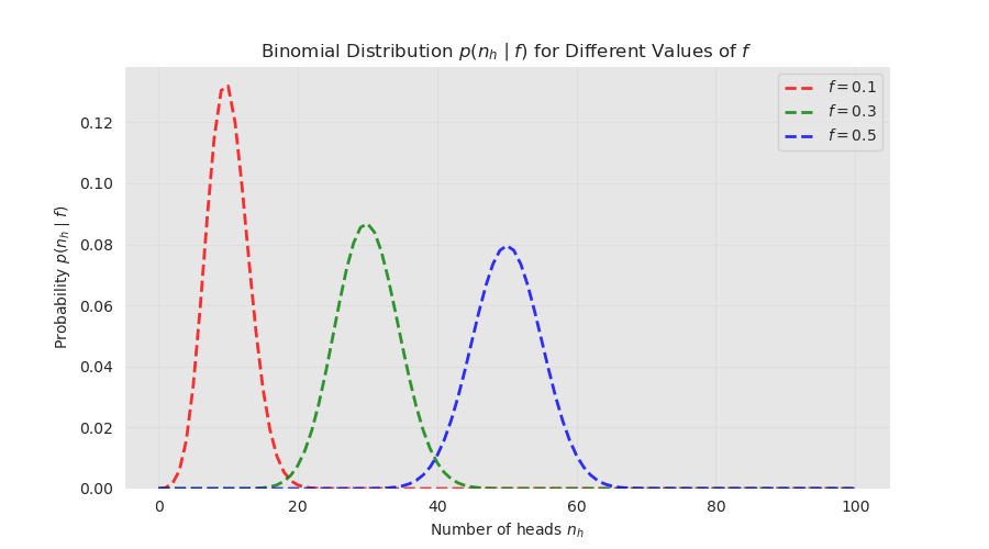
The figure shows the probability distribution of the number of heads for a fixed number of tosses \(n=100\) using three probabilities \(f \in \{0.1, 0.3, 0.5\}\). For a fixed \(n\) both the expected value and variance depend only on the probability \(f\).
Bayes Theorem
Now after motivating our choice for the Binomial model, we go back again to the main task of estimating the unknown parameter \(f\). In other words, we would like to compute the posterior distribution \(p(f\mid n_h)\), that is the probability of \(f\) given the observed heads \(n_h\). In a Bayesian setting, the posterior is given by Bayes' theorem:
\[ p(f \mid n_h) = \frac{p(n_h\mid f)p(f)}{p(n_h)} \]
With \(p(n_h\mid f)\) being the likelihood function of observing a number of heads, which quantifies how plausible different values of \(f\) are under the model given the observations. The term \(p(f)\) is the prior, and it encodes our prior belief on the value of \(f\) before any observations are made. Lastly, \(p(n_h)\) is the evidence, and it corresponds to a normalization factor ensuring that the posterior is a proper probability distribution.
The likelihood function is the Binomial likelihood
\[ p(n_h \mid f) = \binom{n}{n_h}f^{n_h}(1-f)^{n-n_h} \]
To get analytical results we choose a conjugate prior, namely the Beta distribution,
\[ p(f) = \frac{1}{B(\alpha, \beta)} f^{\alpha-1}(1-f)^{\beta-1}, \quad \alpha, \beta > 0. \]
where \(B(\alpha, \beta)\) is the Beta function and it plays the role of a normalization factor. It can be expressed in terms of the Gamma function \(\Gamma(\cdot)\):
\[ B(\alpha, \beta) = \frac{\Gamma(\alpha)\Gamma(\beta)}{\Gamma(\alpha+\beta)} \]
and the Gamma function is related to the factorial by
\[ \Gamma(n) = (n-1)!, \qquad n \in \mathbb{N},\quad n > 0 \]
The parameters \((\alpha, \beta)\) control the concentration and the spread of our prior belief on the value of \(f\).
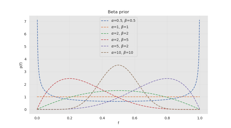
For example the values \((1, 1)\) correspond to an uninformative prior, where the distribution assigns equal weight to all the possible values of \(f\), meaning before making any observations we are unsure what value the parameter takes. On the other hand \((10, 10)\) concentrates around the value \(f=0.5\), reflecting a strong prior belief that the coin is fair.
The last term of the equation, the evidence \(p(n_h)\), is the marginal probability of the number of heads obtained by integrating over all the possible values of \(f\):
\[ p(n_h) = \int_{0}^{1} p(n_h\mid f)p(f)\,df \]
It is fairly easy to compute the evidence over one parameter.
\[ \begin{align} p(n_h) &= \int_{0}^{1} p(n_h|f)p(f)\,df \\ &= \int_{0}^{1} \binom{n}{n_h} f^{n_h}(1-f)^{n-n_h}\frac{1}{B(\alpha, \beta)} f^{\alpha-1}(1-f)^{\beta-1}df \\ &= \binom{n}{n_h} \frac{1}{B(\alpha, \beta)}\int_{0}^{1}f^{n_h+\alpha-1}(1-f)^{n-n_h+\beta-1}df \\ &= \binom{n}{n_h} \frac{B(n_h+\alpha, n-n_h+\beta)}{B(\alpha, \beta)}. \end{align} \]
Note that, since we chose a conjugate prior it is not necessary to compute the integral explicitly, since we know for sure that the posterior will have the same functional form as the prior with different parameters. The final expression of the posterior is then:
\[ p(f|n_h)= \frac{1}{B(n_h+\alpha,\; n-n_h+\beta)} f^{n_h+\alpha-1}(1-f)^{n-n_h+\beta-1}. \]
For \(n=50\) observations generated using the true parameter \(f_{true}=0.6\), and using a uniform Beta prior \((1,1)\), we get:
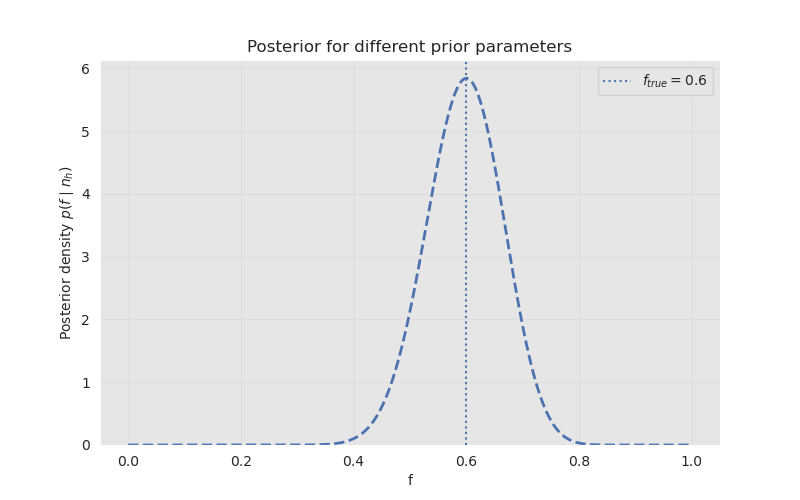
The figure shows that the posterior distribution is concentrated near the true value of the parameter \(f_{true}\). The value at the peak corresponds to the mode of the posterior distribution, which is also the maximum a posteriori estimate.
Monte Carlo Markov Chain Simulations
Usually, computing the normalization factor \(p(n_h)\) is intractable. In such cases we resort to numerical methods, where we sample from the posterior:
\[ p(f\mid n_h)\propto f^{n_h+\alpha-1}(1-f)^{n-n_h+\beta-1} \]
Then we compute the necessary metrics from the generated samples. A common set of algorithms that can be used are called Markov Chain Monte Carlo simulations (MCMC). PyMC provides a simple-to-use interface that performs MCMC simulations using a set of modern sampling algorithms.
We start first by generating synthetic data with \(n\) observations and a true probability \(f_{true}=0.6\).
import numpy as np
import matplotlib.pyplot as plt
import pymc as pm
import arviz as az

SEED = 127

rng = np.random.default_rng(seed=SEED)
size = 50
f_true = 0.6

X = rng.binomial(n=1, p=f_true, size=size)
n_h = X.sum()
print(f"Random sequence: {X}")
print(f"Number of heads: {n_h}")
Then we define the model that will take both the chosen prior and likelihood.
alpha, beta = 1, 1

with pm.Model() as coin_model:
    f = pm.Beta("f", alpha=alpha, beta=beta)
    X_obs = pm.Binomial("X_obs", n=size, p=f, observed=n_h)

    trace = pm.sample(
        tune=1000,
        draws=1000,
        chains=4,
        cores=-1,
        return_inferencedata=True
    )
The trace object contains all the necessary information we need about the sampled posterior, which we can access using the arviz library.
We can retrieve the values of the generated samples from the trace:
f_samples = trace.posterior["f"].values.flatten()Let us visualize the sampled posterior along with the analytical posterior.
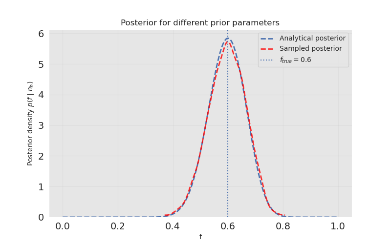
The sampled posterior closely resembles the closed form. However, for this case it is an overkill; the true power of PyMC comes when the models we are dealing with are more complex.
Additionally, let us get the mean and the standard deviation from the summary.
summary = az.summary(trace)
print(f"mean {summary['mean']}")
print(f"std {summary['sd']}")
mean f 0.597
Name: mean, dtype: float64
std f 0.068
Name: sd, dtype: float64