Introduction to Supervised Learning
Introduction
This blog post serves as a light introduction to supervised learning. It introduces the basic ideas behind the field. For a deeper discussion, check out the references section. It assumes knowledge of basic linear algebra, real analysis, and probability.
Workflow
At its core, supervised learning is teaching an algorithm patterns through examples. The examples by which the algorithm is trained are in the form of labeled data, where each sample has an observation and an associated value (target or label). The training process happens iteratively until convergence. After training, the performance of the model is assessed by checking its predictions on previously unseen data.
Data
The key difference between supervised learning and other fields of machine learning is that it relies on labeled data. Formally, a labeled dataset is a set of \(N\) tuples of independent observations \(X_i\) and dependent labels \(y_i\). Each observation vector \(X_i\) contains \(p\) independent features. A supervised learning algorithm solves regression if the target values are continuous or classification if they are discrete.
\[ \mathcal{D} = \{(\mathbf{X}_i, y_i)\}_{i=1}^{N} \]
\(\mathbf{X}_i\) is the observation vector for sample \(i\), each entry of the vector represents a unique feature. \(y_i\) is the measured target value of sample \(i\). For example, a student’s attendance record can be represented as features, and the target is whether the student passed or not.
To check generalization, the dataset is divided into two disjoint subsets: training and testing data, used at different stages of the workflow. The training set usually contains \(80\%\) of the data (\(|\mathcal{D}_{train}|=M\)), and the remaining \(20\%\) are assigned to the test set (\(|\mathcal{D}_{test}|=N-M\)). This way we can check whether the algorithm really learned the underlying patterns or just memorized the training examples (overfitting).
Ideal Model
The targets are assumed to be generated from an unknown generative process \(f(\mathbf{X})\). Supervised learning approximates it with a parameterized model \(g(\mathbf{X};\theta)\). The observations \(\{X_i, \dots, X_N\}\) can be arranged into a design matrix of \(N\) rows (samples) and \(p\) columns (features), \(\mathbf{X} \in \mathbb{R}^{N \times p}\), and the targets into a vector \(\mathbf{y}\) with \(N\) elements.
\[ \mathbf{y} = f(\mathbf{X}) \]
However, in real settings the targets will contain measurement noise. The model then aims to uncover the process \(f(\mathbf{X})\) despite noise, and makes predictions \(\mathbf{\hat{y}}\):
\[ \mathbf{\hat{y}} = g(\mathbf{X};\theta) \] The model can take any functional form depending on the assumed relationship of the data. In simple cases a linear model is enough to uncover the patterns within the data, in more complex cases artificial neural networks are employed to identify non-linear patterns.
A good model is that which approximates the observed data well, and predicts well outputs of new unseen data. It does so by identifying the optimal parameters \(\mathbf{\hat{\theta}}\) that make the model close enough to the true generative process \[ g(\mathbf{X}; \mathbf{\hat{\theta}}) \approx f(\mathbf{X}) \]
Cost Function
The cost function \(\mathcal{C}\) measures how well the model predicts the labels based on the observations. It computes the distance between predictions \(\mathbf{\hat{y}}\) and true values \(\mathbf{y}\). In other words, it measures how far is the model from the true generative process
\[ \mathcal{C}(\mathbf{\hat{y}}, \mathbf{y}_{true}) = \sum_{i=1}^{M'} \ell(\hat{\!y}, y_i) \]
Here, \(\ell(\hat{y}_i, y_i)\) is the cost of a single sample. The costs are additive because the dataset contains independent elements. During training this is called the in-sample error \(E_{in}\), and during testing the out-of-sample error \(E_{out}\).
\[ E_{in}(\mathbf{\hat{y}}, \mathbf{y}) = \frac{1}{M} \sum\limits_{i=1}^{M}\ell(\hat{y}_i, y_i), \quad E_{out}(\mathbf{\hat{y}}, \mathbf{y}) = \frac{1}{N-M} \sum\limits_{i=1}^{N-M}\ell(\hat{y}_i, y_i) \] \(E_{in}(\mathbf{\hat{y}}, \mathbf{y})\) is used during training to fit the parameters of the model to the data, whereas, \(E_{out}(\mathbf{\hat{y}}, \mathbf{y})\) is used after trainign to assess the generalization power of the model on new unseen data.
For regression, a widely used cost function is the mean squared error (MSE):
\[ E_{in}(\mathbf{\hat{y}}, \mathbf{\mathbf{\hat{y}}}) = \frac{1}{M} \sum_{i=1}^{M}\left(\hat{y}_i - y_i\right)^2 \] It measures the mean squared distance between the predicted and true label values. Squaring the differences penalizes predictions that deviate substantially while rewarding predictions that are closer to the true values. To identify the optimal set of parameters the in-sample error \(E_{in}(\mathbf{\hat{y}}, \mathbf{y})\) should be minimized with respect to the parameters. \[ \mathbf{\hat{\theta}} = \arg\min\limits_{\theta} E_{in}(\mathbf{\hat{y}}, \mathbf{y}) \]
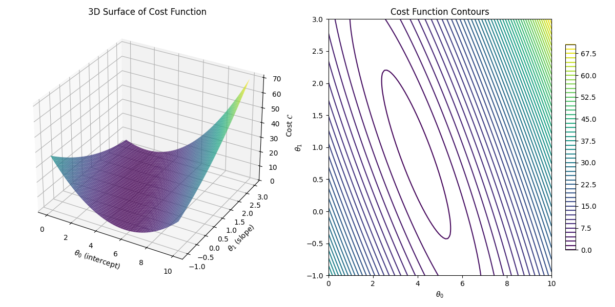
From a physics perspective, the cost function can be thought of as the Hamiltonian of the system, where the ground state corresponds to the set of parameters that minimize the cost function and capture the underlying patterns in the data.
Optimization: Gradient Descent
Gradient descent is an iterative algorithm for minimizing the cost function. Starting from an initial guess \(\theta_0\), it updates the parameters in the opposite direction of the gradient until convergence:
\[ \theta_{t+1} = \theta_t - \eta \nabla_{\theta} \mathcal{C}(\mathbf{\hat{y}}, \mathbf{y}) \]
Here \(\eta\) is the learning rate controlling the step size, \(\mathcal{C}(\mathbf{\hat{y}}, \mathbf{y})\) is the gradient of the cost function with respect to the parameters. Parameters \(\theta_t\) are updated iteratively until convergence.

It is important to choose the appropriate learning rate \(\eta\). If the learning rate is too small, say \(\eta=0.001\) gradient descent algorithm will require many more iterations to converge
On the other hand if the learning rate is too high \(\eta =1.00\), gradient descent will diverge

Linear Regression
Linear regression assumes a linear relationship between features and targets: \[ y_{i\ell} = \sum_{j=1}^{p} x_{ij}\, \omega_{j\ell} + b_{\ell} + \epsilon, \quad i \in \{1,\dots, N\}, \quad \ell \in \{1, \dots, k\} \] where \(x_{ij}\) is the \(j\)-th feature of sample \(i\), \(\omega_{j\ell}\) is the true weight, \(b_{\ell}\) is the bias, and \(\epsilon\) is noise.
A linear model estimates \(\hat{y}_{i\ell}\) by varying parameters \(\theta_{j\ell}\): \[ \hat{y}_{i\ell} = \sum_{j=1}^{p} x_{ij}\, \theta_{j\ell} + b_{\ell} \]
The optimal parameters solve: \[ \widehat{\theta} = \arg\min\limits_{\theta_{j\ell} \in \mathbb{R}} \mathcal{C}(\mathbf{\hat{y}}, \mathbf{y}) \]
For visualization, we consider the simple case of one feature (\(p=1\)), one target (\(k=1\)), and MSE as the cost function.
Python Implementation
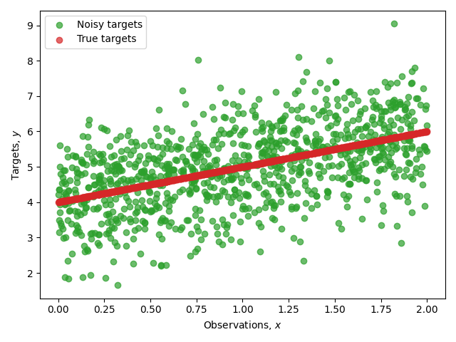
Noisless labels are assumed to be generated from the true linear model \(f(x)\)
\[
f(x) = a x + b
\]
Where \(a\) is the slope, and \(b\) is the intresept. Then, by adding measurement noise we get the measured labels
\[
y = f(x) + \epsilon, \quad \epsilon \sim \mathcal{N}(0, 1)
\]
The goal is to find a linear model \(g(x; \theta) = \theta_0 x + \theta_1\) that approximates the generating
process \(f(x)\) well, in generlizes to unseen data.
We start first by generating \(1000\) synthetic continuous data points in the interval \([0, 2]\). Then to target values we add standard Gaussian noise to each point generated,
with the paramters being \(a=1.00\), and \(b= 2.00\)
          import numpy as np

          # We start first by fixing the seed by reproducing the results
          seed = 127
          # We initialize a random number generator
          rng = np.random.default_rng(seed=seed)

          # We fix the True parameters
          a, b = 2.0, 1.0

          # Then we generate synthetic data
          X = 2 * rng.random(1000)            # Random samples in [0, 2]
          epsilon = rng.normal(0, 1.0, size=1000)  # Gaussian noise
          y_noisy = a * X + b + epsilon
Next step is to split the dataset into training and testing. We do that by shuffling the incidences of the data and we assign \(80\%\) of them to the training data, and the remaining \(20\%\) to the test data.
        # Split into train/test
        train_ratio = 0.8
        N = len(X) # Full size of the data
        train_size = int(train_ratio * N) # The training portion

        indices = np.arange(N) # We get the indecies of the original data
          rng.shuffle(indices) # We then randomly shuffle the indices
        train_idx, test_idx = indices[:train_size], indices[train_size:] # Then we split
        # the indeices into training/testing indices
        # We slice the training/testoing potions
        X_train, X_test = X[train_idx].reshape(-1, 1), X[test_idx].reshape(-1, 1)
        y_train, y_test = y_noisy[train_idx].reshape(-1, 1), y_noisy[test_idx].reshape(-1, 1)

        # Add bias column
        X_train_b = np.c_[np.ones((X_train.shape[0], 1)), X_train]
        X_test_b = np.c_[np.ones((X_test.shape[0], 1)), X_test]
Then, we initialize the parameters to a random values, the learning rate to \(0.1\) and the number of iteration
to \(100\).
          theta = rng.normal(size=(2, 1))  # Random initialization
          n_iter = 100 # Fix the number of iterations
          lr = 0.1 # Fix the learning rate
          m_train = len(y_train) # Get the training data size
          cost_history = [] # Intilize an empty list to store iteration cost values
Last step is to learn the parameters. At each step we compute the gradient of the cost with respect to the
parameters, then we update
the value of the parameters based on the value of the gradient. We repeat this process for the \(100\) steps.
and
then we print the final estimation of the parameters to the screen.
        # Gradient Descent
        for _ in range(n_iter): # We iterate
          # Compute the gradient with respect to the parameters
            gradients = (2/m_train) * X_train_b.T.dot(X_train_b.dot(theta) - y_train)
            # Update the paramters
            theta -= lr * gradients
            # Compute the cost function
            cost = (1/m_train) * np.sum((X_train_b.dot(theta) - y_train)**2)
            # Append the cost function
            cost_history.append(cost)
        # Get the value of the paramters
        theta_0, theta_1 = theta.ravel()
        print(f"Estimated parameters: theta_0 = {theta_0:.2f}, theta_1 = {theta_1:.2f}")
Results
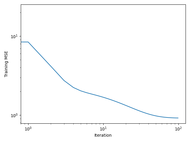
After \(100\) iterations, the estimated parameters are: \[ \hat{\theta_0} \approx 2.00, \quad \hat{\theta_1}\approx 1.00 \] These are very close to the true parameters \(a=2.0\) and \(b=1.0\).
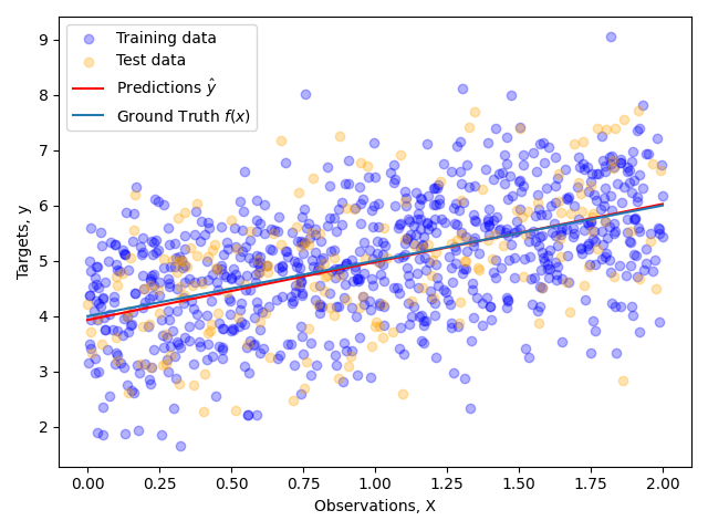
The figure shows the outputs of the true model vs the predictions of the linear model, where the blue circles correspond to the training data points and the yellow ones are the testing data. The predictions closely match the ground truth, and the cost function converges within the first 100 iterations.
Conclusion
This post touched on the basic concepts of supervised machine learning. From how data is structured, to how the cost function measures performance, to how gradient optimizes the parameters. Then they were applied to the simple case of linear regression, where the model learned the true generative process behind the noisy measurements. However, this only scratches the surface. Real world applications are more complicated, yet they all build on the concepts presented in this blog.