Sample Space Reducing Process
Introduction
Many phenomenon are governed by a power law, where some characteristic of the system remains unchanged under re-scaling. Language is an example of such a system, where it has been observed empirically that the frequency of a word in a large corpus is inversely proportional to its rank, following Zipf's law \[ p(rank) \propto rank^{-1} \] Many models have been designed to explain the emergence of scaling in language. In this article, I will explore the sample-space reducing process model, which has been showen to produce perfect Zipf's law.
Sample Space Reducing Process
The sample space reducing process \(\phi\) is a stochastic process characterized by a shrinking sample space \(\Omega_t\). Initially, it contains a set of \(N\) ordered states \(\Omega_0 = \{N,N-1,\dots, 1\}\), each with a prior probability \(\pi_i\) of appearing. The process starts at the highest possible state \(X_0 = N\). At each discrete time step \(t>0\), the process jumps randomly to a lower state \(X_{t+1} < X_{t}\), following two rules:
- Only downward jumps are allowed, \(\mathcal{P}(X_{t+1}=i \mid X_t=j) = p(i \mid j)\)
- The process stops/restarts at the lowest state, \(X_T = 1\)
After every jump, the sample space \(\Omega\) shrinks, making the possible jumps more constrained:
\[ |\Omega_0| > |\Omega_{X_t}| > \dots > |\Omega_{X_T}| \]
This setup reflects how language is produced. When a word is chosen in a text, the next words are constrained by the language’s grammar, semantics, and pragmatics. For instance, the sentence Colorless green ideas sleep furiously is grammatically correct, but semantically nonsensical. In this sense, the sample space of possible words shrinks with each word chosen.
Using a uniform prior probability of state occurance \(\pi_i=\dfrac{1}{N}\), and uniform transition probability over the lower states \(p(i\mid j) = \dfrac{1}{j-1}\), we can show that the probability of state visits \(\mathcal{P}(X_{t>0} = i) =p(i)\) follows an exact Zipf's law
\[ p(i) = i^{-1} \]Numerical Simulation
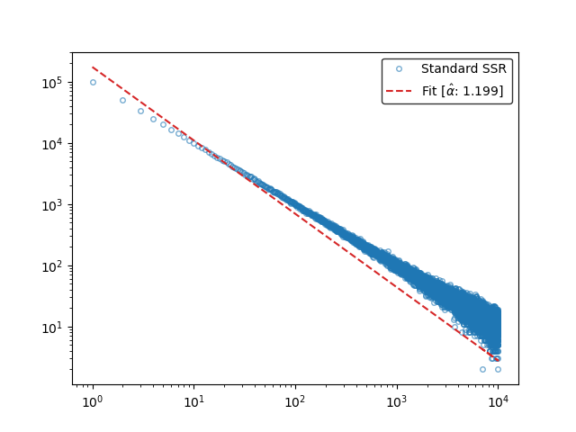
Numerical simulations of the process using \(N=10^4\) states using \(M=10^6\) restarts, show that the state visits frequency indeed follow Zipf's law.
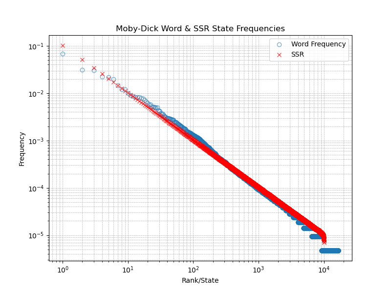
Plotting the state visits frequency \(N=10^4\) states for \(M=10^6\) restarts along with word count of the words from Moby Dick
Conclusion
Despite its simplicity SSR processes provide a simple yet powerful explaination of the emergence of Zipf's law in language. By modeling how the space of possible words shrinks over time.